Some elements of nonlinear elasticity of growing
materials
Michael H. Köpf
January 8, 2015
A very good introduction to nonlinear elasticity can be found in the book by Fu
and Ogden [FO01]. A necessary starter to dive into elasticity theory is certainly the
classical textbook by Landau and Lifshitz [LL70].
In the following, the component notation ci = Aijbj with Einstein summation
over repeated indices is preferred over the notation c = A⋅b, because the latter has to
be translated to the former for every actual calculation, anyway.
1 Basic definitions
The elastic deformation can quantified by comparison of the deformed state
 to a reference state
  . We denote the coordinates in the reference
frame by xi(
. We denote the coordinates in the reference
frame by xi( ) and use Xi(
 ) for the coordinates in the current state
.
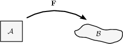
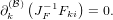
Further, we introduce a mapping F that relates the coordinates of identical
material points in A to the corresponding coordinates in B (see Fig. 1).
) for the coordinates in the current state
.
Further, we introduce a mapping F that relates the coordinates of identical
material points in A to the corresponding coordinates in B (see Fig. 1).
In order to simplify our notation, we introduce the shorthands ∂i() := ∂∕∂xi()
and ∂i() := ∂∕∂xi() for the partial derivatives with respect to the coordinates in
both frames. We define the deformation gradient tensor F by
 | (1) |
and introduce the symbol JF = |F| for its determinant. The
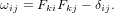
deformation of the solid is quantified by the strain ω defined as
 | (2) |
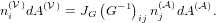
Nanson’s formula
In order to relate the oriented area element dAi() in frame to dAi() in frame
, we consider infinitesimal volume elements in both frames and and use
dxi() = Fijdxj():
 | (3) |
and
 | (4) |
From these two formulas we conclude
| JFdAi() = dA
k()F
ki | |
|
| ⇔ | JF ildAi() = dA
l()
ildAi() = dA
l() | |
|
| ⇔ | JF ilni()dA() = n
i()dA().
ilni()dA() = n
i()dA(). | (5) |
Analogously, we find
 | (6) |
Helpful relations
A few non-obvious identities can be found using Nanson’s formula and very
simple geometric arguments. Consider an arbitrary closed surface δω of some volume
ω in the reference frame .
 | (7) |
Since we can choose the surface ∂ω arbitrarily, we find
 | (8) |
In other words: in the sum ∂k() and JF-1Fki commute. Analogously, we can show
that
 | (9) |
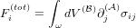
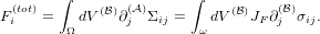
Three different stress tensors
The surface force per unit area on a vector area element dA() in the current
frame is expressed by the Cauchy stress Σij. Using relation (5) we can translate
this to a force per unit area on a vector area element dA() in the reference frame
.
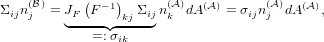 | (10) |
where we have defined the first Piola-Kirchhoff stress σ. The inverse relation
is
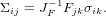 | (11) |
Note, that unlike the Cauchy stress Σ, the first Piola-Kirchhoff stress σ is not
symmetric.
Both ΣdA() and σdA() are force vectors in the current frame . Using F, we
can map it to the reference configuration and obtain
 ijΣjknk()dA() =
 | 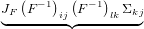 =: silnl()dA() =: silnl()dA() | |
|
| = |  =: siknk()dA() =: siknk()dA() | |
|
| = | sijnj()dA() | (12) |
where we defined the second Piola-Kirchhoff stress s. The inverse relations
are
 | (13) |
Note, that ∂j()Σij on the one hand and ∂j()σij and ∂jsij on the other hand are
force densities with respect to different volumina and therefore differ by a factor of
JF. This can be easily seen by noting that
 | (14) |
and
 | (15) |
Relation of the Piola-Kirchhoff stresses to the elastic free energy
In Hookean elasticity, where, the Cauchy stress is the derivative of the elastic
free energy density per unit volume  el with respect to the linear strain
ωij(lin) = ui,j + uj,i:
el with respect to the linear strain
ωij(lin) = ui,j + uj,i:
 | (16) |
In nonlinear elasticity, the second Piola-Kirchhoff stress takes the role of the
Cauchy stress:
 | (17) |
The first Piola-Kirchhoff stress is given by the derivative of ∂el with respect to the
deformation gradient tensor Fij:
| σij | =  = =   = =  skl skl = =   Fik Fik | |
|
| = Fikskj. | (18) |
In the last step, we have used the symmetry of the second Piola-Kirchhoff stress
s.
2 Elasticity and growth
When the considered material is growing, for example because it is a biological tissue
consisting of proliferating cells, one has to seperate the deformation due to growth
from elastic deformation. This is basically the distinction between growth of a spring
(that might be caused by uniform thermal expansion) versus extension of the spring
by external forces. To make this distinction quantitative, seperate the deformation
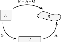
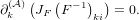
gradient tensor F into a product of the two tensors G and A as proposed by
Rodriguez et al. [RHM94] yielding
 | (19) |
where the growth tensor G describes the deformation due to growth and A describes the elastic part
of the deformation .
We can then distinguish not only between the reference state and the current
deformed state , but also define the virtual state  , that describes the grown but
otherwise undeformed material (see Fig. 2).
, that describes the grown but
otherwise undeformed material (see Fig. 2).
Analogously to the case without growth, we use the shorthands ∂i() := ∂∕∂xi(),
∂i() := ∂∕∂xi(), and ∂i( ) := ∂∕∂xi() for the partial derivatives with respect to
the different coordinate frames and define JF = |F|, JG = |G|, and JA = |A|. Elastic
deformation is deformation from to , only. Therefore, we can for the
moment forget about the frame and consider the reference state. We
can then define the virtual Piola-Kirchhoff stress σ() that translates the
force per unit area in the frame to a force per unit area in the frame
as
) := ∂∕∂xi() for the partial derivatives with respect to
the different coordinate frames and define JF = |F|, JG = |G|, and JA = |A|. Elastic
deformation is deformation from to , only. Therefore, we can for the
moment forget about the frame and consider the reference state. We
can then define the virtual Piola-Kirchhoff stress σ() that translates the
force per unit area in the frame to a force per unit area in the frame
as
 | (20) |
Since the physical force is the same, no matter which frame we choose, the following
two equalities have to hold:
 | (21) |
Using the transformation of the spatial
derivative
∂j() = (G-1)kj∂k() one can use Nanson’s formula (5) applied to , , and G to
find
 | (22) |
When we insert this result into eq. (21), we obtain
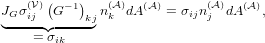 | (23) |
and have thus established the relation between the Piola-Kirchhoff stresses σij and
σij().
References
[Cow04] Stephen C. Cowin. Tissue growth and remodeling. Annu. Rev.
Biomed. Eng., 6(1):77–107, July 2004.
[FO01] Y. B. Fu and R. W. Ogden. Nonlinear Elasticity: Theory and
Applications. Cambridge University Press, Cambridge, 2001.
[LL70] L. D. Landau and E. M. Lifshitz. Theory of Elasticity. Pergamon
Press, New York, 2nd edition, 1970.
[RHM94] Edward K. Rodriguez, Anne Hoger, and Andrew D. McCulloch.
Stress-dependent finite growth in soft elastic tissues. Journal of
Biomechanics, 27(4):455–467, April 1994.